Next: Results
Up: ke3
Previous: Event selection
The event selection described in the previous section results in selected
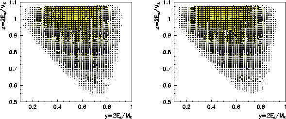
54K events in 1999 data and 79K events in 2001 data. The distribution of
the events over the Dalitz plot is shown in Fig.6. The variables
 and
and
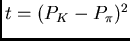
 , where
  ,
,  are the
energies of the electron and
are the
energies of the electron and  in the kaon c.m.s are used. The
background events, as MC shows, occupy the perepherial part of the plot.
in the kaon c.m.s are used. The
background events, as MC shows, occupy the perepherial part of the plot.
Figure 6:
Dalitz plots
 for
the selected
for
the selected
 events after the 2-C fit.
Left- 1999 statistics, Right- 2001 statistics.
events after the 2-C fit.
Left- 1999 statistics, Right- 2001 statistics.
 |
The most general Lorentz invariant form of the matrix element for the
decay
 is [11]:
![\begin{displaymath}
M= \frac{G_{F}sin\theta_{C}}{\sqrt{2}} \bar u(p_{\nu}) (1+ \...
...}}
\sigma_{\alpha \beta}P^{\alpha}_{K}P^{\beta}_{\pi}]v(p_{l})
\end{displaymath}](img75.png) |
(1) |
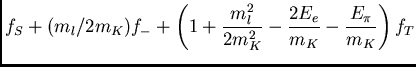
It consists of scalar, vector and tensor terms.
 are the functions of
 . In the Standard Model (SM)
the W-boson exchange leads to the pure vector term. The "induced"
scalar and/or tensor terms, due to EW radiative corrections are negligibly
small, i.e the nonzero scalar/tensor form factors indicate a physics
beyond SM.
. In the Standard Model (SM)
the W-boson exchange leads to the pure vector term. The "induced"
scalar and/or tensor terms, due to EW radiative corrections are negligibly
small, i.e the nonzero scalar/tensor form factors indicate a physics
beyond SM.
The term in the vector part, proportional to  is reduced(using Dirac
equation) to a scalar formfactor. In the same way, the tensor term is reduced to
a mixture of a scalar and a vector formfactors. The redefined
is reduced(using Dirac
equation) to a scalar formfactor. In the same way, the tensor term is reduced to
a mixture of a scalar and a vector formfactors. The redefined  (V),
(V),
 (S) and the corresponding Dalitz plot
density in the kaon rest frame(
(S) and the corresponding Dalitz plot
density in the kaon rest frame(
 ) are [12]:
In case of Ke3 decay one can neglect the terms proportional to
 ;
;  . Then, assuming linear dependance of
on t:
. Then, assuming linear dependance of
on t:
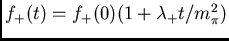 and real constants
 ,
,  we get:
The procedure for the experimental extraction of the parameters
 , , starts from the subtraction of the MC
estimated background from the Dalitz plots of Fig.6. The background
normalization was determined by the ratio of the real and generated
, , starts from the subtraction of the MC
estimated background from the Dalitz plots of Fig.6. The background
normalization was determined by the ratio of the real and generated
 events. Then the Dalitz plots were
subdivided into 20
events. Then the Dalitz plots were
subdivided into 20  20 cells.
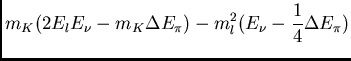
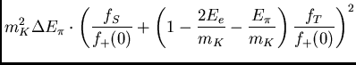
The background subtracted distribution of the numbers of events in the cells
(i,j) over Dalitz plots, for example, in the case of
simultanious extraction of and
20 cells.
The background subtracted distribution of the numbers of events in the cells
(i,j) over Dalitz plots, for example, in the case of
simultanious extraction of and
 ,
was fitted with the function:
,
was fitted with the function:
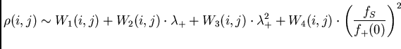 |
|
|
(4) |
Here  are MC-generated functions, which are build up as follows:
the MC events are generated with constant density over the Dalitz plot and
reconstructed with the same program as for the real events. Each event
carries the weight w determined by the corresponding term in formula 3,
calculated using the MC-generated values for y and z.
The radiative corrections according to [13] were taken into account.
Then is constructed by summing up the weights of the events in
the corresponding Dalitz plot cell. This procedure allows to avoid the
systematics errors due to the "migration" of the events over the Dalitz plot
because of the finite experimental resolution.
are MC-generated functions, which are build up as follows:
the MC events are generated with constant density over the Dalitz plot and
reconstructed with the same program as for the real events. Each event
carries the weight w determined by the corresponding term in formula 3,
calculated using the MC-generated values for y and z.
The radiative corrections according to [13] were taken into account.
Then is constructed by summing up the weights of the events in
the corresponding Dalitz plot cell. This procedure allows to avoid the
systematics errors due to the "migration" of the events over the Dalitz plot
because of the finite experimental resolution.
Next: Results
Up: ke3
Previous: Event selection
Alexander V.Inyakin
2002-03-27